Model Overview

1. Model overview:

Model Predictive Control (MPC) is a classic control algorithm widely used in control engineering. It models the controlled system to predict outputs from control inputs, formulates an objective function for control input and error, and solves an optimization problem for a control sequence. Typically, only the first value of the solved sequence is output for the current iteration, then rolling optimization continues at the next step to avoid error accumulation and improve responsiveness to dynamic changes.
MPC has two core problems: modeling and optimization. Optimization is usually formulated as a standard problem and solved with available toolboxes, whereas modeling requires analysis of the specific task.

Trajectory tracking receives trajectory or path data from upstream Decision-Making and Planning, typically timestamped coordinates. It outputs vehicle steering/front-wheel angle and throttle opening. This example mainly addresses lateral trajectory tracking; longitudinal output is directly expressed as speed.

2. File descriptions:

• reference.mat contains reference-trajectory data: timestamp t_ref, x coordinate x_ref, and y coordinate y_ref. The reference trajectory is typically generated by the upstream Decision-Making and Planning module.
• Sim_Demo.slx is a Simulink file for graphical programming and simulation. It includes the overall control framework and the controlled-plant model.
• MPC_sFunction.m is the controller S-function file containing the MPC control algorithm code.
• evaluator.mlx contains post-processing code, including plots for trajectories, errors, and vehicle-state curves, as well as an animation demonstration.

0. Preparation:

• This project runs in MATLAB R2022a or later and requires the complete Simulink toolbox.

1. Run the file:

• Double-click Sim_Demo.slx and wait for Simulink to start.
• Click Run to start the simulation.

• After the run, the working directory contains reference_processed.mat and Sim_result.mat. reference_processed.mat stores intermediate initialization data produced by the controller to reduce repeated calculations; Sim_result.mat stores simulation results.

2. Post-process the results:

• After simulation, visualize the results by double-clicking evaluator.mlx.
• On the Live Editor tab, click Run Section in sequence to view the results of each section.

1. Simulation model:

• The simulation model consists of two main parts: (1) the controlled system and (2) the controller.

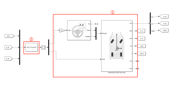
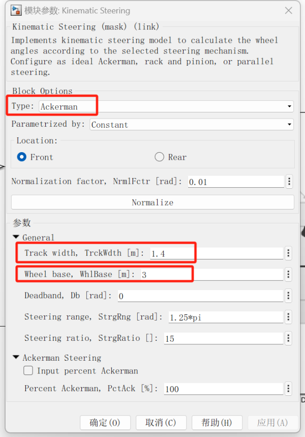
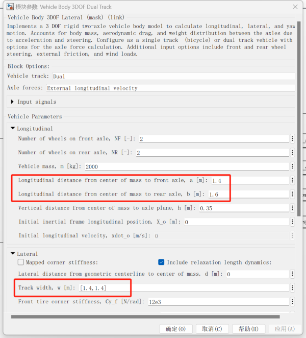
• The controlled objects use the kinematic steering system model and the two-track body three-degree-of-freedom model in the Vechicle Dynamic Blockset in the Simulink toolbox. Because this project mainly focuses on lateral control, in the three-degree-of-freedom model of the body, the longitudinal vehicle speed is a direct input. The kinematic steering system model type is selected as Ackerman steering relationship. The wheel width, TrckWdth and wheelbase in the parameter settings need to be consistent with those in the vehicle model to ensure that the steering system matches the vehicle. The wheelbase is the sum of the distances from the center of mass to the front and rear axles: WhlBase = a + b.

• controllerWritten with s-function, input the current yaw angle of the vehicle and the xy coordinates in the geodetic coordinate system. See the specific code and parameters later.

2. MPC Controller:

• The MPC controller is written in the form of s-function

• t is time; x is the iteration state variable; u is the input of the system; sys is the variable returned by each function, and the values ​​returned in different modules are different;
• mdlInitializeSizes is the initialization function;
• mdlDerivatives(t,x,u) is a differential iteration function. sys returns the derivative of the state variable in this module to model differential equation relationships;
• mdlOutputs(t,x,u) output function, sys returns output in this module.

3. Post-processing Program:

Post-processing programs need to be used to visualize results including calculation and drawing of actual trajectories and errors, trajectory tracking effect animation, and vehicle status parameters.
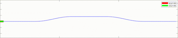
Number change curve, etc. The specific code is relatively simple and I won’t go into details. The trajectory control effect animation is shown below.