Model Overview

1. Model overview:

Proportional-integral-derivative control, or PID control, is simple, practical, and widely used. Most vehicle control algorithms in use today include PID control. With few parameters, PID can achieve good control performance through repeated manual tuning even when the system model is not fully known.

Longitudinal Control: although longitudinal trajectory control would ideally control longitudinal position, longitudinal and lateral position errors are typically coupled in practice. Controlling longitudinal position alone is therefore of limited value; Longitudinal Control in autonomous vehicles mainly refers to regulating longitudinal speed.

2. File descriptions:

• reference.mat contains reference-trajectory data: timestamp t_ref, x coordinate x_ref, and y coordinate y_ref. The reference trajectory is typically generated by the upstream Decision-Making and Planning module.
• Sim_Demo.slx is a Simulink file for graphical programming and simulation. It includes the overall control framework and the controlled-plant model.
• MPC_sFunction.m is the controller S-function file containing the MPC control algorithm code.
• evaluator.mlx contains post-processing code, including plots for trajectories, errors, and vehicle-state curves, as well as an animation demonstration.

0. Preparation:

• This project runs in MATLAB R2022a or later and requires the complete Simulink toolbox.
• Download and extract the project, then set the MATLAB working directory to this folder.

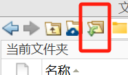
• Alternatively, copy the files in the folder into the current directory.

1. Run the file:

• Double-click Sim_Demo.slx and wait for Simulink to start.
• Click Run to start the simulation.

• After the run, the working directory contains reference_processed.mat and Sim_result.mat. reference_processed.mat stores intermediate initialization data produced by the controller to reduce repeated calculations; Sim_result.mat stores simulation results.

2. Post-process the results:

• After simulation, visualize the results by double-clicking evaluator.mlx.
• On the Live Editor tab, click Run Section in sequence to view the results of each section.

1. Simulation model:

• The simulation model has two main parts: (1) the controlled plant and (2) the controller. The controller is implemented as an S-function, while the controlled vehicle is MATLAB’s three-degree-of-freedom vehicle model, shown below.

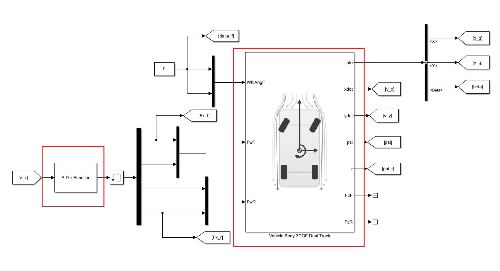
• The controlled plant is a three-degree-of-freedom vehicle model configured with longitudinal force as input.

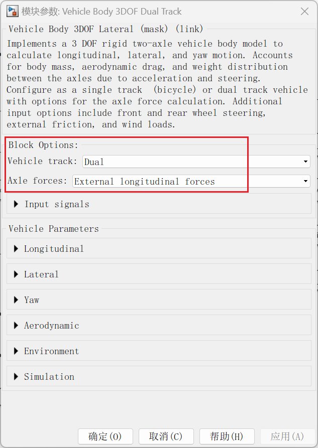
• For Longitudinal Control, lateral motion is not considered: the vehicle follows a straight line and its front-wheel steering angle remains 0.

3. PID algorithm:

PID control works by feeding back error. The error and its integral and derivative are supplied to the controlled system; while error remains, the PID controller computes an input to correct it until the error is eliminated and the control objective is achieved.

For a unified format, the PID control algorithm is also written using s-function, and its main function is

• In this example, speed error is defined as

in,is the desired vehicle speed, which is calculated in the initial function

• Weighting the proportional, integral, and derivative terms of the error yields the desired input acceleration.

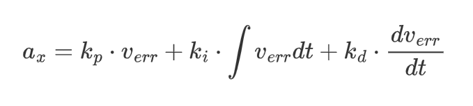
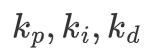in,are proportional, integral and differential coefficients respectively.

• In the S-function, discrete states can be used to calculate the integral and derivative processes above.

in,is the sampling time, and the integral is expressed as follows by accumulation:

Because computing the integral and derivative requires variables from the previous time step, the S-function mdlUpdate module can be used.

3. Longitudinal-force allocation:

The PID controller produces longitudinal acceleration, which can also be interpreted as throttle opening or total longitudinal force. Different vehicles may require different input signals. In this example, the plant requires longitudinal forces applied at all four wheels, which are simply allocated according to vertical loads to make full use of road adhesion.

The total longitudinal force is:

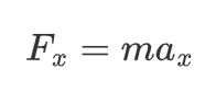
For simplicity, distribution can be based on static loads
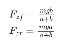
Therefore, the vertical force on the front and rear axles is:

The longitudinal forces on the front and rear axles are:

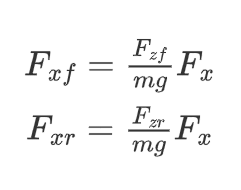
This process is implemented in the output function of the S-function.

4. Result evaluation and visualization:

• Longitudinal tracking is commonly simplified to speed tracking. Its metric is therefore longitudinal speed-tracking control error; the mean longitudinal speed-control error can be defined as:

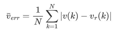
In this case, the average longitudinal speed control error is=0.0808 m/s。

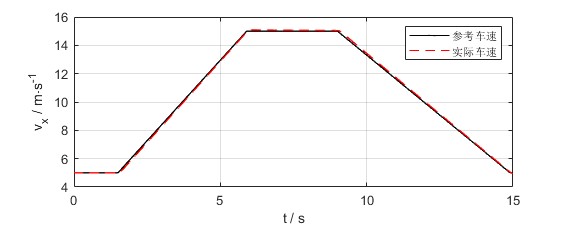
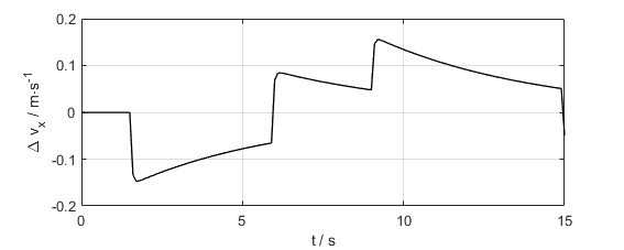
• The longitudinal speed-tracking and error curves are shown below.

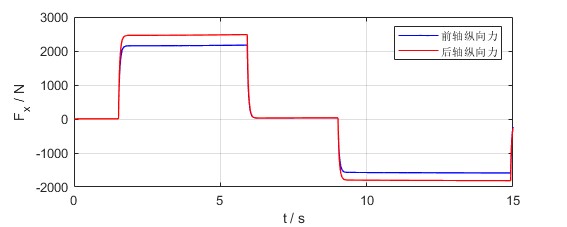
• The longitudinal-force input curve is shown below.

• Animation