Model Overview

1. Model overview:

LQR (Linear Quadratic Regulator) produces an optimal linear state-feedback control law and readily forms closed-loop optimal control. It converts linear-system control into a quadratic optimization problem. For an infinite-horizon regulator, theory yields an analytic expression for the solution, so online computation is limited.

Trajectory tracking receives trajectory or path data from upstream Decision-Making and Planning, typically timestamped coordinates. It outputs vehicle steering/front-wheel angle and throttle opening. This example mainly addresses lateral trajectory tracking; longitudinal output is directly expressed as speed.

2. File descriptions:

• reference.mat contains reference-trajectory data: timestamp t_ref, x coordinate x_ref, and y coordinate y_ref. The reference trajectory is typically generated by the upstream Decision-Making and Planning module.
• Sim_Demo.slx is a Simulink file for graphical programming and simulation. It includes the overall control framework and the controlled-plant model.
• LQR_sFunction.m is the controller S-function file containing the LQR control algorithm code.
• evaluator.mlx contains post-processing code, including plots for trajectories, errors, and vehicle-state curves, as well as an animation demonstration.

0. Preparation:

• This project runs in MATLAB R2022a or later and requires the complete Simulink toolbox.
• Download and extract the project, then set the MATLAB working directory to this folder.

• Alternatively, copy the files in the folder into the current directory.

1. Run the file:

• Double-click Sim_Demo.slx and wait for Simulink to start.
• Click Run to start the simulation.

• After the run, the working directory contains reference_processed.mat and Sim_result.mat. reference_processed.mat stores intermediate initialization data produced by the controller to reduce repeated calculations; Sim_result.mat stores simulation results.

2. Post-process the results:

• After simulation, visualize the results by double-clicking evaluator.mlx.
• On the Live Editor tab, click Run Section in sequence to view the results of each section.

1. Simulation model:

As shown, the simulation model has a controller and a controlled plant. The controller is implemented as an S-function, while the controlled vehicle is MATLAB’s three-degree-of-freedom vehicle model, shown below:

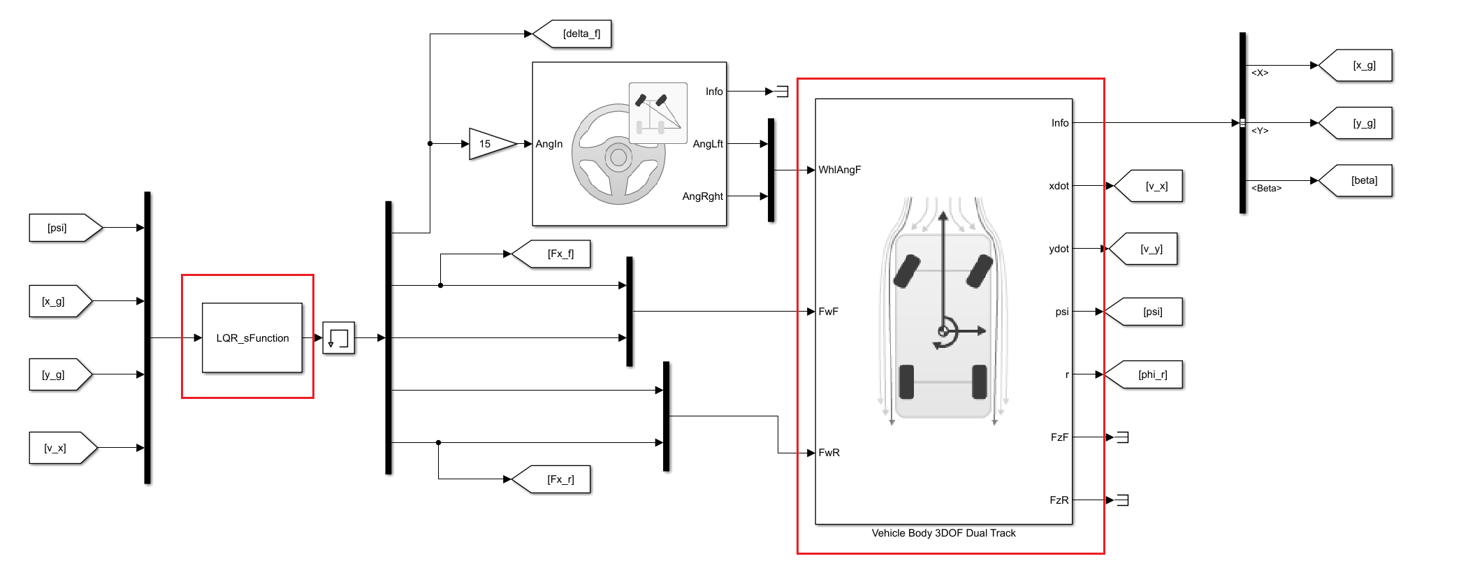
• The setting parameters of the combination control are as shown below, and settings need to be made in the red box.
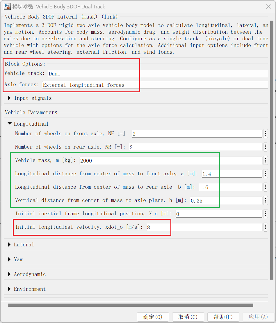
  • Set the vehicle as a dual-track model, that is, the left and right wheels can be given different parameters, and the Ackermann angle relationship needs to be considered when turning. The longitudinal force given to the four wheels on the drive can theoretically realize the longitudinal force distribution strategy front and rear and left and right.
  • Set the initial speed of the vehicle to 8m/s to prevent problems caused by sudden changes in the starting target.
• Read and note the parameters in the green box for later controller design.

2. LQR controller:

• The LQR controller is implemented as an S-function and mainly uses output and initialization modules. Its main function is

An LQR controller starts from a linear model, defines an objective for inputs and errors, and constructs an optimization problem. Because the input is a sequence and the output is an objective value, this is a variational optimization problem. Its quadratic integral objective can be solved by calculus of variations; the optimum is obtained from a Riccati differential equation. For an infinite-horizon, linear time-invariant regulator, this reduces to an algebraic Riccati equation, so the controller only needs to solve that equation online and use simple matrix operations to compute control inputs.

• First establish the control model. In global coordinates, using the rear-axle center as the reference point, the vehicle kinematic equations can be written as

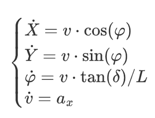
in the formula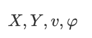is the system status,is the control quantity
LQR control, as the name implies, needs to be applied to the linear model. Therefore, it is necessary to linearize the model and place the nonlinear equation at the reference pointTaylor expansion to first order obtains a linearized model of the disturbance quantity

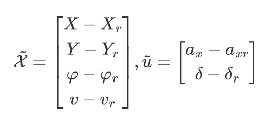
• Define perturbations:

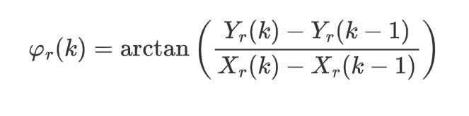
• Among the reference quantities, \(X_r\) and \(Y_r\) can be directly indexed through time, and the reference yaw angle calculation formula is:

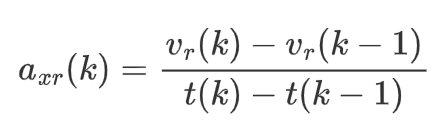
• The reference speed calculation formula is

• The reference acceleration is further differentiated based on the vehicle speed.

• The reference front wheel rotation angle is obtained through the third equation of the kinematic model

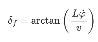
The turning vehicle is regarded as a uniform circular motion instantaneously, so there is

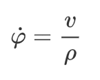
in,is the radius of instantaneous circular motion, that is, the radius of curvature of the trajectory. Substituting the formula into simplified form, we get

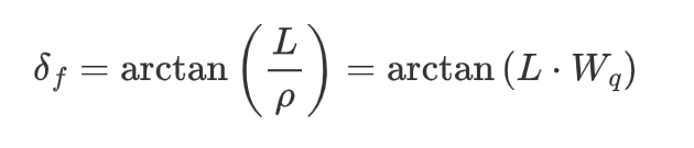
Among them, \(W_q\) is the curvature of the trajectory, and the expression is

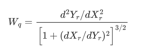
These reference values can be computed in the initialization function.

In order to ensure accurate control tracking, only \(X-X_r \rightarrow 0, Y-Y_r\rightarrow 0, v-v_r\rightarrow 0\) is required, so the output equation can be defined as:

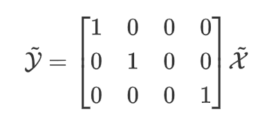
The system can therefore be written in state-space form.

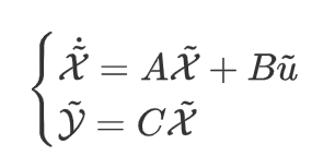
The current control objective is that during the entire control process, the error of the controlled quantity \(\tilde{\mathcal{Y}}\) should be as small as possible, and the input should not be too large, so the objective function can be written as

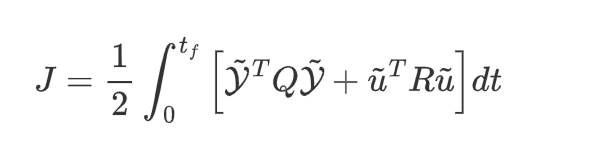
Among them, \(Q\) is the symmetric positive definite matrix of \(3\times3\). Usually we place the weight on the diagonal. The position of the diagonal corresponds to the controlled quantity. The greater the weight, the greater the proportion of the error corresponding to the controlled quantity in the objective function. The algorithm will give priority to reducing the modified part of the error. \(R\) is the symmetric positive definite matrix of \(2\times2\). The weights are usually placed on the diagonal, corresponding to the two input quantities. The larger the weight, the algorithm prioritizes reducing that part of the input.

At this point, the control problem becomes that it is necessary to obtain a suitable control function \(\tilde u\) to act on the constrained slave system, and ultimately minimize the above objective function. This is a constrained functional extremum problem. In order to solve this problem, the Lagrange multiplier method is first used to transform the constrained optimization problem into an unconstrained extreme value problem, and then the variation method is used to solve it. At the same time, after substituting \(\tilde{\mathcal{Y}}=C\tilde{\mathcal{X}}\), the augmented objective function is

In the formula, \(\lambda\) is the introduced costate.
To sort it out, let the Hamiltonian function be:

Then the objective function becomes

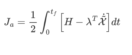
Use the variational formula to obtain the variation of the objective function as

To show the difference, \(\Delta\) is a variational symbol. When \(t_f \rightarrow \infty\), the final state needs to be stable to the target value, so \(\Delta \tilde{\mathcal{X}}(t_f)=0\) the truncation equation is naturally satisfied. In order to satisfy the extreme value variation\(\Delta J_a=0\), it needs to satisfy

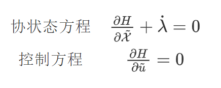
After substituting, put the state equation into

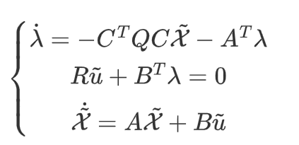
Through observation, it is found that these equations are linear mapping relationships at each moment, so the precondition is set to

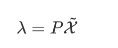
Here, the mapping relationship \(P\) is allowed to be time-varying.

Substituting into the previous three equations to sort out, we get

After adding the above preconditions, the compiled equation must always hold true to prove that the added conditions are correct, then the Ricati differential equation is

Furthermore, we observe that the parameters of the system are all time-invariant and are infinite-time regulators. Therefore, assuming that \(P\) is also time-invariant\(\dot P=0\), the Ricati differential equation is reduced to an algebraic equation.

Ricati algebraic equations can be solved manually through the undetermined coefficient method. Ricati equations can be directly solved using the `care` function in MATLAB. The calling format is `[P,~,~]=care(A,B,Q1,R)`
Among them\(Q_1=C^TQC\)

After solving to obtain \(P\), the control input is

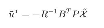
Encapsulate the LQR-solver procedure above in a function to obtain

3. Longitudinal-force distribution:

Finally, convert incremental control inputs back to actual control inputs.

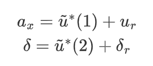
Longitudinal acceleration (throttle opening) can be converted into wheel longitudinal forces or torques depending on the plant model input. Here, the input is wheel longitudinal force, so it must be allocated. The total longitudinal force can be calculated as

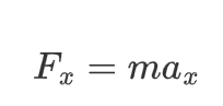
Among them, \(m\) is the mass of the vehicle
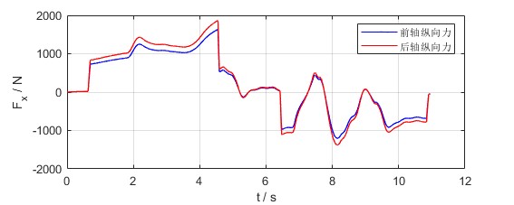
The longitudinal force distribution of the front and rear axles can be distributed in proportion according to the vertical force of the front axle, which is conducive to giving full play to the road adhesion coefficient. The vertical force on the front and rear axes is divided into two parts: static and dynamic. The static vertical force is determined by the position of the center of mass, and the dynamic vertical force is caused by longitudinal acceleration. The amount of load transfer caused by dynamic acceleration is

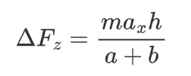
Among them, \(h\) is the height of the center of mass, \(a\) and \(b\) are the distances from the center of mass of the vehicle to the front and rear axles.
Therefore, the vertical force on the front and rear axles is

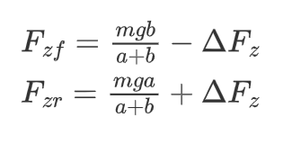
The longitudinal forces on the front and rear axles are:

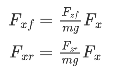
This process is implemented in the output function of the S-function.

4. Post-processing results:

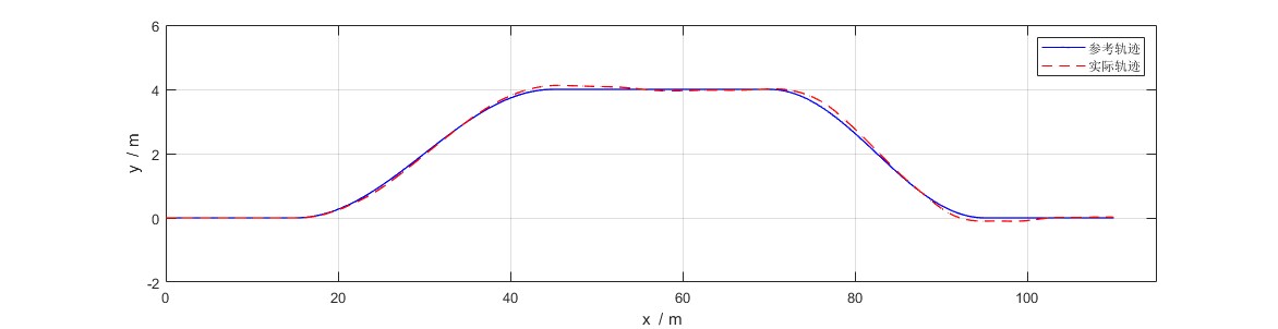
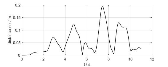
• Combined Control applies both lateral and longitudinal control. Tracking error can be represented by the mean distance between reference and actual positions at corresponding times:

In this example, the average position tracking error is \(\bar{dis}_{err}=0.0554\mathrm{m}\)

• The path-tracking results and error curves are shown below:

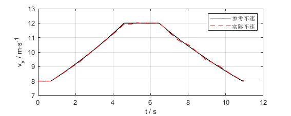
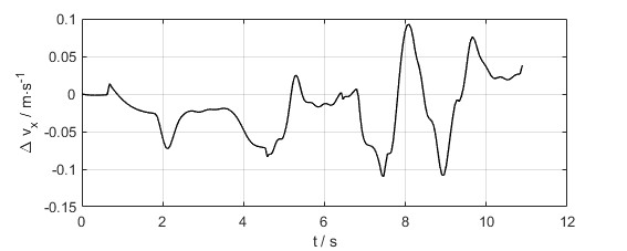
• The speed-tracking results and error curves are shown below.

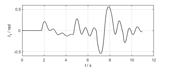
• The input front-wheel angle and front/rear axle longitudinal-force inputs are shown below.

• The trajectory-tracking animation is shown below.